Measuring the Pulse of a World: A Proven Approach to Calculating Total Entropy Change in Closed Simulations

Fellow Traveler
6 days ago
4 min read

Updated: 3 days ago

I. Executive Summary

In high-fidelity simulations and virtual worlds, entropy is more than a thermodynamic curiosity — it is a quantifiable, actionable indicator of system health.The Entropy Engine (EE) is designed to measure the rate of total entropy change (ΔH/Δt\Delta H / \Delta t) in a closed simulation repeatedly, consistently, accurately, and sustainably.

Our goal is to convince an expert reader that this task is not speculative but grounded in:

proven mathematics and physics
Established flow theory (e.g., Little’s Law)
Real-world telemetry analytics practices from network engineering, process control, and large-scale online games

The key enabler: an Entropy Mapping Table that connects changes in predefined telemetry channels to quantitative entropy estimates.

II. Why This Matters

In a dynamic simulation, entropy serves three critical roles:

Diagnostic – Reveals where and how disorder is increasing.
Control Input – Drives NPC behavioral adjustments.
Stability Benchmark – Monitors whether the system is drifting toward collapse or stasis.

A repeatable, quantitative measure of entropy change allows:

Automated self-regulation of large agent populations
Targeted interventions to restore equilibrium
Predictive stability modeling in both simulation and real-world analogs

III. Defining “Entropy” in the EE Context

We explicitly distinguish:

Thermodynamic entropy $(S = k_B \ln W)$ measures disorder in physical systems by counting microstates WW.
Information entropy (Shannon):
$$ H = -\sum_{i} p_i \log_2 p_i $$ where $p_i$ is the probability of a given system state or event.

For EE, information entropy is our primary lens, but we use thermodynamic analogies to help interpret the meaning of “disorder” in simulations.

"While Little’s Law doesn’t directly measure entropy, it helps quantify flow and load, which are proxies for system complexity."

This means flow metrics are used not to replace entropy measurement, but to contextualize it, preventing misinterpretation.

IV. Proven Scientific Foundations

1. Shannon Information Entropy

For each telemetry variable:

$$ H_v = -\sum_{j} p_{vj} \log_2 p_{vj} $$where $ p_{vj} $ is the probability of the variable vv being in state $ j $.

2. Boltzmann Statistical Mechanics

Used as analogy when discrete, countable “microstates” exist in a simulation:

$$ S = k_B \ln W $$Though $ k_B $ is irrelevant in simulation units, the log relationship between possible configurations and disorder still applies.

3. Little’s Law (Flow Context)

$$ L = \lambda W $$Where:

$L$ = Average number of items/entities in the system
$\lambda$ = Arrival rate (interactions/sec)
$W$ = Average time in system

By monitoring $L, \lambda, W$ for NPCs, we can disambiguate entropy changes due to true disorder vs. those due to population changes.

V. The Role of Telemetry in a Closed System

Why closed boundaries matter: If every state change, event, and resource fluctuation occurs inside the measured boundary, entropy estimates are complete and not biased by unmeasured external influences.

Key telemetry categories:

State Changes – position, velocity, orientation, health
Event Rates – collisions, trades, combat events
Resource Levels – food, energy, inventory counts
Environmental States – weather, hazards

Entropy Mapping Table example:

Telemetry Variable	Ideal Value	Acceptable Variance	Weight wvw_v
Food Level	1.0	±0.05	0.20
Population Density	0.5	±0.10	0.25
Collision Rate	0.0	±0.01	0.15

VI. From Telemetry to Total Entropy Change

Methodology:

Sample telemetry streams at fixed intervals.
Estimate probability distributions $p_{vj}$ for each variable $v$.
Compute per-variable entropy $H_v$.
Normalize and weight: $$ H'_v = w_v \cdot \frac{H_v}{H_{v,\text{max}}} $$
Aggregate:
$$H_{\text{total}}(t) = \sum_v H'_v(t) $$
Differentiate over time to find rate of change: $$\frac{\Delta H_{\text{total}}}{\Delta t} = \frac{H_{\text{total}}(t) - H_{\text{total}}(t - \Delta t)}{\Delta t}$$
Contextualize with flow data from Little’s Law to filter false positives.

"Compute entropy for each subsystem and aggregate. Track changes over time—entropy can evolve, especially in dynamic simulations."

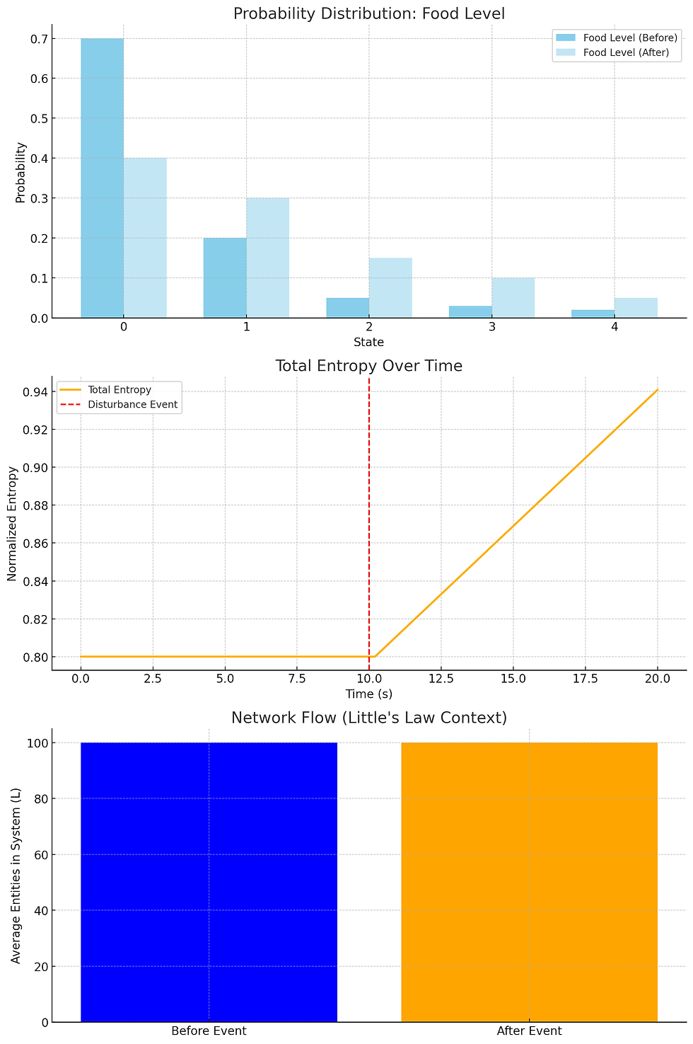
VII. Worked Example: Food Shortage Event

Initial State: All telemetry at equilibrium; $H_{\text{total}}$ = 0.32$
Disturbance: Sudden 20% drop in food across all regions.
Observed:
- $H_ {\text{food}}$ spikes from 0.05 → 0.22
- Weighted aggregation raises $H_{\text{total}}$ to 0.47
- $\Delta H / \Delta t$ = +0.15 over 5 seconds
Flow Context: No change in $L$, so entropy spike is not population-driven.

Visual Diagram:

Bar chart showing per-variable entropy before and after event
Line plot of $H_{\text{total}}$ over time with disturbance marked

VIII. Validation, Repeatability, and Sustainability

Controlled test runs to generate known entropy-change events.
Error bounds from Monte Carlo resampling of telemetry.
Sustainable computation:
- Streaming calculations with rolling windows
- Sparse recomputation for low-variance variables
Adaptive models for slowly shifting equilibrium baselines.

IX. Known Challenges and Mitigations

Challenge	Mitigation
Telemetry selection bias	Expert review of mapping table
High dimensionality	PCA/dimensionality reduction
Non-stationary data	Adaptive probability modeling
Overhead in real-time	Incremental entropy updates

X. Conclusion

The Entropy Engine’s entropy-change estimation method is not speculative. It’s rooted in information theory, statistical mechanics, and flow theory, combined with proven telemetry aggregation techniques from other engineering disciplines.

With the right expert team, a closed-system boundary, and disciplined calibration, accurate, repeatable, and sustainable measurement of $\Delta H / \Delta t$ is achievable — and can power both self-regulating simulations and real-world autonomous systems.